Week 3: Diffusion equations in 1D
\[ \renewcommand{\vec}[1]{\boldsymbol{#1}} \newcommand{\td}[2]{\frac{\mathrm{d}#1}{\mathrm{d}#2}} \newcommand{\tdd}[2]{\frac{\mathrm{d}^2#1}{\mathrm{d}#2^2}} \newcommand{\pd}[2]{\frac{\partial#1}{\partial#2}} \newcommand{\pdd}[2]{\frac{\partial^2#1}{\partial#2^2}} \]
Overview
This week we enter the realm of numerically solving partial differential equations (PDEs). We will focus on one of the most important PDEs of them all: the diffusion equation. By using finite differences to discretise space, the diffusion equation can be converted into a system of ODEs. There are two main ways to solve this ODE system.
The explicit Euler method is the simplest method, and it can be extended to nonlinear problems relatively easily. However, the method only works if the time step \(\Delta t\) is sufficiently small. This means that a large number of time steps may be required to obtain a solution.
The implicit Euler method is more complex because it involves solving a system of algebraic equations at each time step. Howver, larger values of the time step \(\Delta t\) are usually possible. In fact, for the linear diffusion equations, the implicit Euler method is unconditionally stable, meaning it will work for any time step size \(\Delta t\). The need to solve an algebraic system of equations at each time step comes at a high computational cost. Hence, there is a tradeoff between being able to take fewer time steps to obtain a numerical solution and the higher computational cost per time step.
Supplementary material
Use the links below to find:
Exercises
Use the explicit Euler method to solve the linear diffusion equation without a source term \[ \pd{u}{t} = D\pdd{u}{x}. \] Set the boundary conditions to \(u(a,t) = 0\) and \(u(b,t) = 0\) and the initial condition to \[ u(x,0) = \sin\left(\frac{\pi (x - a)}{b - a}\right). \]
The exact solution to the problem is given by \[ u(x, t) = \exp\left(-\frac{D \pi^2 t}{(b-a)^2}\right)\sin\left(\frac{\pi (x - a)}{b - a}\right). \] which you can use to test your code.
Use the implicit Euler method to solve the problem in Exercise 1, using the same analytical solution to validate your code.
Explicit vs implicit Euler. In this exercise, you will compare the performance of the two Euler methods by timing your codes. Find out more about how to time your code here. Consider the diffusion equation and boundary conditions from Exercise 1. Take \(a = 0\), \(b = 1\), and \(D = 0.1\). Discretise the spatial domain using 31 grid points (\(N = 30\)) and solve the problem until time \(T = 1\).
- Fix the time step to be \(\Delta t = 0.005\). Show that this time step is smaller than the maximum time step that can be used with the explicit Euler method. Solve the problem using the explicit and implicit Euler method. Which method is the fastest and why?
- Increase the time step to \(\Delta t = 0.1\) and solve with the implicit Euler method. How does the speed of the implicit Euler method now compare to the speed of the explicit Euler method with \(\Delta t = 0.005\)? Which of the two methods leads to a more accurate solution when \(t = 1\)?
Extend your code so that it can solve linear reaction-diffusion equations of the form \[ \pd{u}{t} = D \pdd{u}{x} + q(x), \\ \] with two Dirichlet boundary conditions. Use the supplementary notes to find exact solutions that you can use to test your code with.
Solve the Fisher-KPP equation (a nonlinear reaction-diffusion equation) given by \[ \pd{u}{t} = D\pdd{u}{x} + r u (1 - u) \] on the domain \(0 \leq x \leq 10\). The boundary and initial conditions are \[ u(0,t) = 1, \qquad u(10,t) = 0, \qquad u(x,0) = 0. \] You can take \(D = 0.1\) and \(r = 2\). Run your simulation until \(t = 20\) and use 51 grid points (\(N = 50\)). What types of solution do you see?
Hint: there are three ways to solve this problem: (i) using the explicit Euler method, which is the easiest to implement; (ii) using the implicit Euler method, which allows larger time steps to be taken; and (iii) using an implicit-explicit (IMEX) method, which combines the simplicity of explicit Euler with the numerical stability of implicit Euler. Try starting with the explicit Euler or IMEX method.
Coursework-style problem
This problem explores the fluid and solid mechanics of coffee brewing. Consider a fresh layer of coffee grains of height \(H = 10\) mm. The coffee is on placed top of a perforated metal surface that allows water to pass through it. Let \(z\) be an upwards-pointing vertical coordinate such that \(z = 0\) corresponds to the bottom of the coffee and \(z = H\) corresponds to the top of the coffee. At time \(t = 0\), water enters the top surface of the coffee. The water then flows through the coffee grains and leaves through the bottom surface.
The coffee grains form a porous solid that deforms as water flows through it. The flow of water through the solid, along with the gravitational force, generates a pressure gradient. The pressure gradient acts on the solid to deform it. The pressure in the coffee grains, \(p(z,t)\), satisfies the following equation \[\begin{align} \frac{1}{E}\pd{p}{t} = K \pdd{p}{z}. \end{align}\] Here, \(E = 10^4\) Pa is the Young’s modulus and \(K = 5.6 \times 10^{-10}\) m\(^2\) Pa\(^{-1}\) s\(^{-1}\) is the hydraulic conductivity. The Young’s modulus measures the stiffness of the porous solid formed by the coffee grains, and \(K\) characterises how easy it is for fluid to flow through the coffee grains.
The pressure of the coffee is initially at the atmospheric pressure, \(p(z,0) = p_a\), where \(p_a = 101.3\) kPa. The pressure at the bottom of the coffee can be assumed to be equal to the atmospheric pressure, \(p(0,t) = p_a\). To account for the influx of water at the top of the coffee grains, the boundary condition at \(z = H\) is given by \[\begin{align} K \left(\pd{p}{z} + \rho g\right)_{z = H} = F(t) \end{align}\] where \(\rho= 1000\) kg m\(^{-3}\) is the density of wet coffee, \(g = 9.81\) m/s\(^2\) is the gravitational acceleration, and \(F(t)\) represents the flux of water coming into the coffee. We will assume that the flux is given by \[\begin{align} F(t) = \begin{cases} F_0, \quad 0 \leq t \leq 10~\text{s}, \\ 0, \quad t > 10~\text{s}, \end{cases} \end{align}\] where \(F_0 = 2 \times 10^{-5}\) m/s, which represents a 10 second injection of water into the coffee.
Calculate the difference in fluid pressure at the top surface, \(\Delta p = p(H,t) - p_a\) after 5, 10, 15, and 30 s have passed. Answers (to 3 significant figures): 154, 206, 20.6, -83.16 Pa.
Compute the steady-state pressure profile and plot. Recall that the steady-state pressure is obtained by assuming that time \(t\) is very large and that the solution does not depend on time. How does your steady-state profile compared to the pressure you computed from problem 1? Answer: you should find that your time-dependent solution approaches the steady-state solution.
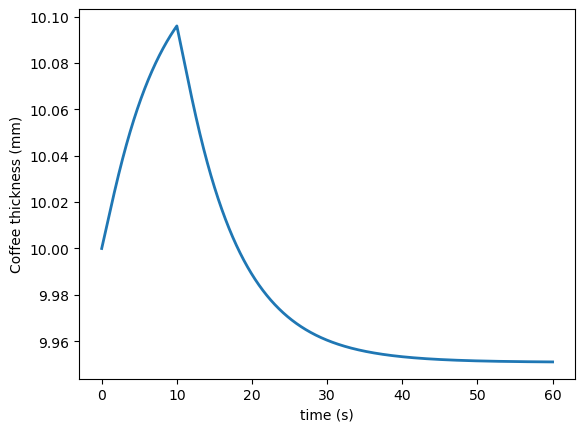
The displacement of the coffee grains, \(u(z,t)\), can be determined from the equation \[\begin{align} \pd{u}{z} = \frac{p-p_a}{E}. \end{align}\] Since coffee cannot pass through the metal surface on which it rests, the displacement at \(z = 0\) is zero, \(u(0,t) = 0\). The deformed thickness of the coffee layer is given by \(h(t) = H + u(H,t)\). Plot how the thickness of the coffee layer changes in time. Is the final thickness of the coffee layer larger or smaller than the initial thickness? Answer: smaller, the coffee layer shrinks.
Answers to selected exercises
3. (a) Explicit Euler is the fastest because the computational cost of each time step is smaller. (b) Implicit Euler is now the fastest because it now requires less time steps. However, the explicit Euler method is the more accurate method because the time step is smaller.
5. See figure below 