Week 4: First-order PDEs in 1D
\[ \renewcommand{\vec}[1]{\boldsymbol{#1}} \newcommand{\td}[2]{\frac{\mathrm{d}#1}{\mathrm{d}#2}} \newcommand{\tdd}[2]{\frac{\mathrm{d}^2#1}{\mathrm{d}#2^2}} \newcommand{\pd}[2]{\frac{\partial#1}{\partial#2}} \newcommand{\pdd}[2]{\frac{\partial^2#1}{\partial#2^2}} \]
Overview
This week we focus on an first-order PDEs. These are PDEs that only involve first-order partial derivatives. Although these are the simplest of all PDEs, they lead to surprising numerical challenges. In particular, the finite-difference discretisation needs to adapt to the sign of the coefficient in front of the spatial derivative (the wave speed). Choosing a numerically stable discretisation requires a consideration of the direction of wave propagation. Adapting the spatial discretisation based on the direction of wave propagation is called upwinding.
In this unit, we will use the upwind scheme to numerically solve first-order PDEs. Although this method is simple, it suffers from numerical diffusion. This leads to the numerical solution artifically spreading out. Moreover, there is also a restriction on the time step that is set by the CFL condition.
Supplementary material
Exercises
Solve the linear advection equation given by \[ \pd{u}{t} + v \pd{u}{x} = 0 \] where \(v\) is a constant. Take the domain to be \(0 \leq x \leq 5\) and \(0 \leq t \leq 4\). Set the initial condition to \(u(x,0) = x / 5\).
- Solve with \(v = 1\) and the boundary condition \(u(0, t) = 0\). Validate your code using the exact solution \[ u(x,t) = \begin{cases} 0, \quad &0 \leq x \leq t, \\ \frac{1}{5}(x - t), \quad &t \leq x \leq 5. \end{cases} \]
- Solve with \(v = -1\) and the boundary condition \(u(5, t) = 1\). Validate your code using the exact solution \[ u(x,t) = \begin{cases} \frac{1}{5}(x + t), \quad &0 \leq x \leq 5 - t, \\ 1, \quad &5 - t \leq x \leq 5. \end{cases} \]
- Use the velocity decomposition to write an upwind scheme that can simultaneously handle both of these cases.
Use exercise 1a to explore the truncation error of the upwind scheme by comparing your numerical approximation to \(u(5,4)\) to the exact value of \(1/5\). Do this in two ways. First, fix the value of \(\Delta t\), vary \(\Delta x\), and compute and plot the truncation error. Then, compute the truncation error by fixing the value of \(\Delta x\) and varying the size of the time step \(\Delta t\). Are the results what you expect? To understand the results, try solving Exercise 3.
Consider again the problem in exercise 1a. Set \(N = 100\) so that \(\Delta x\) is now fixed. Now choose values of \(\Delta t\) so that the CFL number is set to \(C = 0.5\), \(C = 0.8\), and \(C = 1\). On the same axes, plot \(u(x,4)\) for all three cases along with the exact solution. What happens when \(C\) is increased to one? How you can explain the results in term of the truncation error and the numerical diffusion coefficient?
Solve the linear advection equation given by \[ \pd{u}{t} + v(x,t)\pd{u}{x} = 0 \] on the domain \(-1 \leq x \leq 1\). Let the velocity be given by \(v(x, t) = x\). Notice that \(v < 0\) for \(x < 0\) and \(v > 0\) for \(x > 0\). Take the initial condition to be \(u(x,0) = 1 - x^2\). Do boundary conditions need to be imposed for this problem?
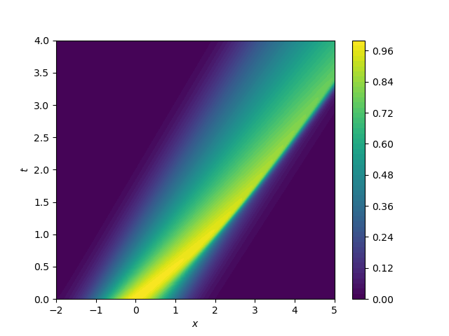
Solve the hyperbolic conservation law \[ \pd{u}{t} + \pd{}{x}\left(j(u)\right) = 0 \] when \(j(u) = u + u^3 / 3\). Take the domain to be \(-2 \leq x \leq 5\) and \(0 \leq t \leq 2\). The initial condition can be set to \(u(x,0) = \exp(-x^2)\). If needed, set \(u = 0\) at the boundaries.
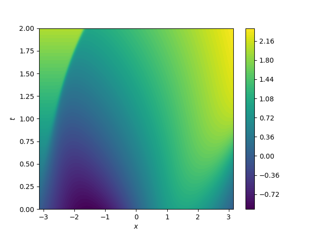
Solve the forced inviscid Burgers’ equation \[ \pd{u}{t} + u \pd{u}{x} = 1 \] over the domain \(-\pi \leq x \leq \pi\) and \(0 \leq t \leq 2\). The initial condition can be set to \(u(x,0) = \sin x\). If boundary conditions are needed, set \(u = t\) at the boundary.
Answers to selected exercises
See figures below
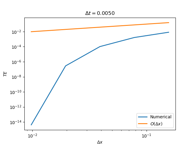
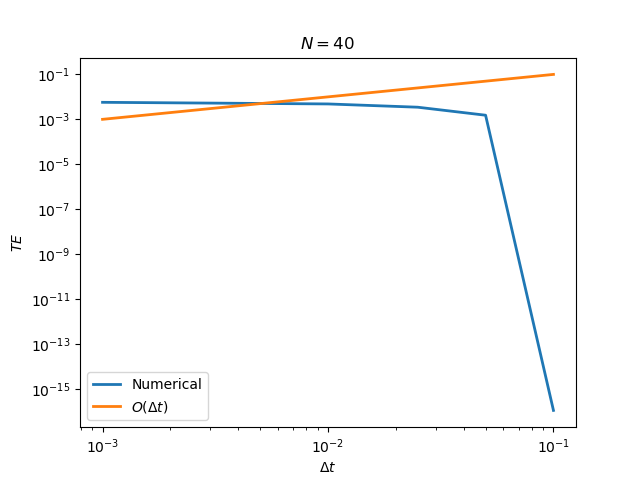
As \(C\) increases to one, the numerical solution becomes more accurate and there is less numerical diffusion. From the formula for the truncation error, we see the numerical diffusion coefficient is proportional to \((1 - C)\). Setting \(C = 1\) therefore eliminates numerical diffusion. Decreasing \(\Delta t\) with a fixed value of \(\Delta x\) means that \(C\) decreases from one, leading to more error, as seen in Exercise 2.
No boundary conditions are needed
See figure below
See figure below